


Often we may need to clean the data using Python and Pandas.
This tutorial explains the basic steps for data cleaning by example:
- Basic exploratory data analysis
- Detect and remove missing data
- Drop unnecessary columns and rows
- Detect outliers
- Inconsistent data
- Irrelevant features
What is Data Cleaning? What is dirty Data?
First let's see what is dirty data:
dirty data is inaccurate, incomplete or inconsistent data
The common features of dirty data are:
- spelling or punctuation errors
- incorrect data associated with a field
- incomplete data
- outdated data
- duplicated records
The process of fixing all issues above is known as data cleaning or data cleansing.
Usually data cleaning process has several steps:
- normalization (optional)
- detect bad records
- correct problematic values
- remove irrelevant or inaccurate data
- generate report (optional)
At the end of the process data should be:
- complete
- up to date
- accurate
- correct
- consistent
- relevant
- normalized
For tidy data
- each observation is saved in its own row
- each variable is saved in its own column
Setup
In this post we will use data from Kaggle - A Short History of the Data-science.
Above you can find a notebook related to 2019 Kaggle Machine Learning & Data Science Survey.
To read the data you need to use the following code:
import kaggle

link = 'eswarankrishnasamy/2019-kaggle-machine-learning-data-science-survey'

kaggle.api.authenticate()
kaggle.api.dataset_download_file(link, file_name='multiple_choice_responses.csv',  path='data/')
The downloaded data can be ready by:
import pandas as pd
pd.read_csv('data/multiple_choice_responses.csv.zip', low_memory=False)
Data looks like:
| Time from Start to Finish (seconds) | Q1 | Q2 | Q2_OTHER_TEXT | Q3 |
|---|---|---|---|---|
| Duration (in seconds) | What is your age (# years)? | What is your gender? - Selected Choice | What is your gender? - Prefer to self-describe - Text | In which country do you currently reside? |
| 510 | 22-24 | Male | -1 | France |
| 423 | 40-44 | Male | -1 | India |
| 83 | 55-59 | Female | -1 | Germany |
| 391 | 40-44 | Male | -1 | Australia |
Step 1: Exploratory data analysis in Python and Pandas
To start we can do basic exploratory data analysis in Pandas. This will show us more about data:
- data types
- shape and size
- missing values
- sample data
The first method is head() - which returns the first 5 rows of the dataset.
To see the first 5 rows and 5 columns we can do: df.iloc[0:5,0:5]
df.head()
The result is truncated for the first 5 columns:
| Time from Start to Finish (seconds) | Q1 | Q2 | Q2_OTHER_TEXT | Q3 | |
|---|---|---|---|---|---|
| 0 | Duration (in seconds) | What is your age (# years)? | What is your gender? - Selected Choice | What is your gender? - Prefer to self-describe - Text | In which country do you currently reside? |
| 1 | 510 | 22-24 | Male | -1 | France |
| 2 | 423 | 40-44 | Male | -1 | India |
| 3 | 83 | 55-59 | Female | -1 | Germany |
| 4 | 391 | 40-44 | Male | -1 | Australia |
Next we can see information about the number of the columns and rows by df.shape:
df.shape
The result is a tuple showing 19718 rows and 246 columns:
(19718, 246)
Similar information we can get by df.info():
df.info()
result:
<class 'pandas.core.frame.DataFrame'>
RangeIndex: 19718 entries, 0 to 19717
Columns: 246 entries, Time from Start to Finish (seconds) to Q34_OTHER_TEXT
dtypes: object(246)
memory usage: 37.0+ MB
Finally we can get more details information about the data values by method describe(). This method will generate descriptive statistics (summarize the central tendency, dispersion and shape of a dataset’s distribution, excluding NaN values).
df.describe()
| Time from Start to Finish (seconds) | Q1 | Q2 | Q2_OTHER_TEXT | Q3 | |
|---|---|---|---|---|---|
| count | 19718 | 19718 | 19718 | 19718 | 19718 |
| unique | 4169 | 12 | 5 | 46 | 60 |
| top | 450 | 25-29 | Male | -1 | India |
| freq | 42 | 4458 | 16138 | 19668 | 4786 |
Step 2: First rows as header read_csv in Pandas
So far we saw that the first row contains data which belongs to the header. We need to change how we read the data with header=[0,1]:
df = pd.read_csv('data/multiple_choice_responses.csv.zip', low_memory=False, header=[0,1])
The above will read the multiline header from the CSV file.
In order to simplify the reading of the data we can drop single level from the multi-index by:
df.droplevel(level=1, axis=1)
Step 3: Data tidying in Pandas
Next we can do data tidying because tidy data helps Pandas's vectorized
operations.
For example column 'Q1' looks like - we need to use the multi-index in order to read the column:
df[('Q1', 'What is your age (# years)?')]
resulted data is:
0        22-24
1        40-44
2        55-59
3        40-44
4        22-24
Can we split that into two columns? It looks like that all values are two numbers separated by '-' hyphen. The best is to confirm that observation by:
df[('Q1', 'What is your age (# years)?')].value_counts()
The last rows shows us one record - 70+ which needs special attention
45-49                           949
50-54                           692
55-59                           422
60-69                           338
70+                             100
dtype: int64
If we perform split operation on rows containing 70+ will result into:
df['Q1'].str.split('-', expand=True)
output
0     70+
1    None
Name: 182, dtype: object
Step 4: Correcting and replacing data in Pandas
Next we can see how to correct the data above. We can do data correction of cases 70+ in two ways:
- replace value of 70+ with something else
- split the column and fill the NaN values
4.1. Replace values in column - Pandas
To replace the values in the column we can use method .str.replace('70+', '70-120', regex=False) as follows:
df['Q1'].str.replace('70+', '70-120', regex=False)
4.2. Fill NaN with string or 0 - Pandas
The other option is to fill the missing values after the split by:
df['max_age'].fillna(120)
we suppose that after the split we created new column 'max_age'
Step 5: Detect NaN values in column Pandas
Now let's see how we can detect NaN values. This will help us drop columns with NaN values.
5.1 Columns which contains only NaN values
To find columns which has only NaN values we can use two methods:
isna()all()
s = df.isna().all()
This will give a new Series with column name and True or False - depending on the NaN values. If a column has only NaN values we will get True.
To find columns which contain NaN values we can use:
s[s == True]
the result is:
Series([], dtype: bool)
There's no column which contains only NaN values
5.2 Detect columns with NaN values
To detect columns which has NaN values we can use:
df.isna().any()
This will result into:
Time from Start to Finish (seconds)    False
Q1                                     False
Q2                                     False
Q2_OTHER_TEXT                          False
Q3                                     False
                                       ...
Q34_Part_9                              True
Q34_Part_10                             True
Q34_Part_11                             True
Q34_Part_12                             True
Q34_OTHER_TEXT                         False
Length: 246, dtype: bool
So columns like 'Q34_Part_9' have NaN values. Columns like 'Q1' don't have NaN values.
Step 6: Drop columns in Pandas
Let's say that we would like to drop columns based on name or NaN values. We can do that in several ways:
6.1 Drop one column by name
Parameters needed to drop columns are axis=1 and inplace=True - which means that operation will affect DataFrame.
df.drop('Q1', axis=1, inplace=True)
6.2 Drop multiple columns by name
We can list several column which to be removed by:
df.drop(['Q1', 'Q2'], axis=1, inplace=True)
6.3 Drop columns with NaN values
Finally we can drop columns which has NaN values:
df.dropna(axis=1, how='any')
We can use parameters like:
how- 'all' or 'any'subset- list of columnstresh- the number of NaN values required to remove the columninplace
Step 7: Detect and drop duplicate rows in Pandas
To detect duplicate values in the DataFrame we can use the method duplicated(). To detect duplicate rows in Pandas DataFrame we can use:
df[df.duplicated()]
This results in 4 duplicated rows:
4 rows × 246 columns
We can use parameter: keep
- first - only the first rows
- last - the last row only
- False - show all rows
For example get indexes of all detected duplications:
df[df.duplicated(keep=False)].index
Int64Index([11228, 12344, 16413, 16547, 16653, 18705, 19258, 19705], dtype='int64')
Since we have 246 columns (answers) it's pretty suspicious that there are full duplications.
We can use method df.drop_duplicates(subset=['Q1']) in order to drop duplicated rows in Pandas:
df.drop_duplicates(subset=['Q1', 'Q2'])
Step 8: Detect outliers in Pandas
We can detect outliers in Pandas in many ways. Here we will cover basic detection of numeric data:
- check stats for the column - min, max and percentiles
- visually by plotting values
Suppose we work with column: 'Time from Start to Finish (seconds)'
We can see the min, max and the percentiles by:
df['Time from Start to Finish (seconds)'].describe()
The result is:
count     19717.000000
mean      14341.281027
std       74166.106601
min          23.000000
25%         340.000000
50%         540.000000
75%         930.000000
max      843612.000000
Name: (Time from Start to Finish (seconds), Duration (in seconds)), dtype: float64
So we have time for the survey from 23 up to 843612 seconds. Probably we can exclude some of them.
Another way to detect outliers is visually by plotting data like:
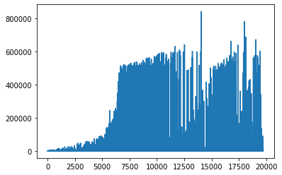
From the image above we can decide what is the threshold which makes sense for us.
Step 9: Detect errors, typos and misspelling in Pandas
Finally let's check how we can detect typos and misspelled words in Pandas DataFrame. This will show how we can work with inconsistent or incomplete data.
For this purpose we are going to read file - 'other_text_responses.csv' which will be df_other. The reason is that it contains free text input.
Let's read the third column of this DataFrame by:
df_other[df_other.columns[3]].value_counts().head(10)
The result is:
Excel              865
Microsoft Excel    392
excel              263
MS Excel            67
Google Sheets       61
Google sheets       44
Microsoft excel     38
Excel               33
microsoft excel     27
EXCEL               25
We can see different variations of the same tool - Excel.
In order to detect similar values we will use Python library difflib:
import difflib
difflib.get_close_matches('excl', ['Excel', 'Microsoft Excel ', 'MS Excel', 'excel'], n=1, cutoff=0.7)
The result of this will be:
['excel']
So we can use Python in order to detect and fix misspelled words.
Code like the one below can help us create new column with corrected values:
import difflib

correct_values = {}
words = df_other["Q14_Part_3_TEXT"].value_counts(ascending=True).index

for keyword in words:
    similar = difflib.get_close_matches(keyword, words, n=20, cutoff=0.6)
    for x in similar:
        correct_values[x] = keyword

df_other["corr"] = df_other["Q14_Part_3_TEXT"].map(correct_values)
Conclusion
In this article, we learned what is clean data and how to do data cleaning in Pandas and Python.
Some topics which we discussed are NaN values, duplicates, drop columns and rows, outlier detection.
We saw all the steps of the data cleaning process with examples. We covered important topics like tidy data and data quality.