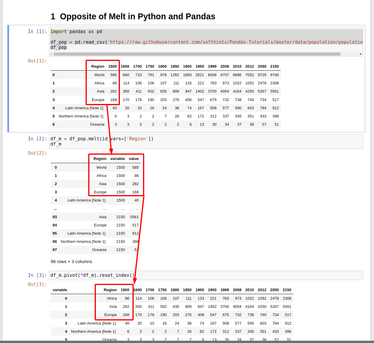
In this short guide, you'll see what is the opposite operation of melt in Pandas and Python. You can find a useful example.
The short answer of the question above is:
df_m.pivot(*df_m).reset_index()
Let's show a detailed example on the above:
import pandas as pd

df_pop = pd.read_csv('https://raw.githubusercontent.com/softhints/Pandas-Tutorials/master/data/population/population.csv')
df_pop
| Region | 1500 | 1600 | 2010 | 2012 | 2050 | 2150 |
|---|---|---|---|---|---|---|
| World | 585 | 660 | 6896 | 7052 | 9725 | 9746 |
| Africa | 86 | 114 | 1022 | 1052 | 2478 | 2308 |
| Asia | 282 | 350 | 4164 | 4250 | 5267 | 5561 |
| Europe | 168 | 170 | 738 | 740 | 734 | 517 |
| Latin America [Note 1] | 40 | 20 | 590 | 603 | 784 | 912 |
In order to demo the opposite of melt operation let's perform melt on the above data:
df_m = df_pop.melt(id_vars=['Region'])
df_m
The DataFrame df_m has the next data inside:
| Region | variable | value |
|---|---|---|
| World | 1500 | 585 |
| Africa | 1500 | 86 |
| Asia | 1500 | 282 |
| Europe | 1500 | 168 |
| Latin America [Note 1] | 1500 | 40 |
| Northern America [Note 1] | 1500 | 6 |
| Oceania | 1500 | 3 |
| World | 1600 | 660 |
| Africa | 1600 | 114 |
| Asia | 1600 | 350 |
So the years which were stored as columns after the melt operation are transformed to rows.
Instead of the initial columns:
Index(['Region', '1500', '1600', '1700', '1750', '1800', '1850', '1900',
       '1950', '1999', '2008', '2010', '2012', '2050', '2150'],
      dtype='object')
after melt operation we end with 3 columns:
- Region - the column on which we do the melt operation
- variable - which is the column name of the old DataFrame
- value - the corresponding value of the first DataFrame
Reverse Melt Operation in Python and Pandas
Now let's reverse the melt which was performed above. We are going to work with DataFrame df_m.
There are several ways of reversing melt operation in Pandas. In this post we will demonstrate the one which uses method pivot and reset_index:
df_m.pivot(*df_m).reset_index()
If you like to get the original DataFrame from you will need to rename the columns by .rename_axis(None, axis='columns'). So the full code will become:
df_m.pivot(*df_m).reset_index().rename_axis(None, axis='columns')
The difference between those two is the name of the index. Without .rename_axis(None, axis='columns') we will get:
Index(['Region', '1500', '1600', '1700', '1750', '1800', '1850', '1900',
'1950', '1999', '2008', '2010', '2012', '2050', '2150'],
dtype='object', name='variable')
with .rename_axis(None, axis='columns') we will have different index name after the pivot.:
Index(['Region', '1500', '1600', '1700', '1750', '1800', '1850', '1900',
'1950', '1999', '2008', '2010', '2012', '2050', '2150'],
dtype='object')

Note: Please note that the index is sorted alphabetically and doesn't match the original sort.
Opposite of melt on few values only
Finally let's see the example when you like to melt or reverse it on a few variables. This can be done by using parameter value_vars of method melt:
df_m = df_pop.melt(id_vars=['Region'], value_vars=['1500', '1600', '1700'])
df_m
result:
| Region | variable | value |
|---|---|---|
| World | 1500 | 585 |
| Africa | 1500 | 86 |
| Asia | 1500 | 282 |
| Europe | 1500 | 168 |
| Latin America [Note 1] | 1500 | 40 |
The reverse operation have additional parameter column:
df_m.pivot(index='Region', columns='variable')['value']
| variable | 1500 | 1600 | 1700 |
|---|---|---|---|
| Region | |||
| Africa | 86 | 114 | 106 |
| Asia | 282 | 350 | 411 |
| Europe | 168 | 170 | 178 |
| Latin America [Note 1] | 40 | 20 | 10 |
| Northern America [Note 1] | 6 | 3 | 2 |


