Pandas vs R - cheat sheet   

This is a Python/Pandas vs R cheatsheet for a quick reference for switching between both. The post contains equivalent operations between Pandas and R. The post includes the most used operations needed on a daily baisis for data analysis.

Have in mind that some examples might differ due to different indexing or updates.

If you want to contribute feel free to suggest changes or additions on GitHub: pandas_r_cheatsheet.csv

Pandas vs R cheatsheet

Setup

Import and package installation

import pandas as pd import numpy as np

library(dplyr) library(ggplot2) # error if missing require(ggplot2) # warning

Import libraries and modules

pip install pandas

install.packages('ggplot2')

install package

https://pypi.org/

https://cran.r-project.org/web/packages/

Search Packages

Data Structures

Pandas Series vs R Array DataFrame comparison

s = pd.Series(np.arange(5))

s <- 0:4 # >

Pandas series vs R vectors

s[0]

s[0]

Get first element of array or Series

df = pd.DataFrame( {'col_1': [11, 12, 13], 'col_2': [21, 22, 23]}, index=[0, 1, 3])

df = data.frame ( col_1 = c(11, 12, 13), col_2 = c(21, 22, 23) ) rownames(df) <- c(0,1,3) # >

Pandas vs R DataFrame

import numpy as np import pandas as pd data = np.random.randn(10, 3) cols = list('abc') pd.DataFrame(data, columns=cols)

data.frame(a=rnorm(10), b=rnorm(10), c=rnorm(10))

Create random DataFrame

Read

Import Data R vs Pandas

df = pd.read_csv('file.csv')

df <- read.csv('file.csv') # >

Read CSV file

pd.read_json('file.json')

library(jsonlite) df <- read_json('file.json') # >

Read JSON file

pd.read_csv('https://example.com/file.csv')

read.csv(url('https://example.com/file.csv'))

Read data from URL

df = pd.read_fwf('delim_file.txt')

df <- read_fwf('delim_file.txt') # >

Read delimited file

Write

Data export - Pandas vs R

df.to_csv('file.csv')

write.csv(df, 'data.csv', row.names=FALSE)

Writes to a CSV file

df.to_json('file.json')

js_file <- jsonlite::toJSON(df2, pretty = TRUE) write(js_file, 'file.json') # >

Writes to a file in JSON format

Inspect Data

Statistics, samples and summary of the data

df.shape

dim(df)

return dimensions

df.head(6)

head(df, 6)

First n rows

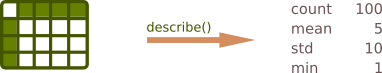
df.tail(6)

tail(df, 6)

Last n rows

df.describe()

summary(df)

Summary statistics

df.loc[:, :'a'].describe()

summary(df[, 'a'])

Describe columns

df['A'].mean()

mean(df[, 'a'])

Statistical functions

df.sample(n=10)

sample_n(df, 10)

Sample n random rows

Select

Select data by index, by label, get subset

df.loc[1:3, :]

df[2:4,]

Select first N rows - all columns

df.loc[[1, 2, 3], :]

df[c(2,3,4),]

Select rows by index

df.loc[:, ['a', 'b']].copy()

copy <-data.frame(df[,c('a','b')]) # >

Select columns by name(copy)

df.loc[:, ['a']]

df[, 'a']

Select columns by name(reference)

df.loc[1:3, ['b', 'a']]

df[2:4, c('b','a')]

Subset rows and columns

df.loc[[3,1], ['b', 'a']]

df[4:2, c('b','a')]

Reverse selection

df[df['a'].isna()]

df[is.na(df$a), ]

Select NaN values

df['a'].dropna()

df[!is.na(df$a), ]

Select non NaN values

Add rows/columns

Add new columns and rows

df['new col'] = df['col'] * 100

df$new <- df[, 'a'] * 100 # >

Add new column based on other column

df['new col'] = False

df$new <-FALSE # >

Add new column single value

df.loc[-1] = [1, 2, 3]

df[nrow(df) + 1,] = c(1,2,3)

Add new row at the end of DataFrame

df.append(df2, ignore_index = True)

rbind(df, df2)

add rows from DataFrame to existing DataFrame

Drop rows/columns/nan

Drop data from DataFrame

s.drop(1)

s[!(s == 1)]

(Series) Drop values from Series by index (row axis)

s.drop([1, 2])

s[!(s %in% c(1,2))]

(Series) Drop values from Series by index (row axis)

df.drop('b' , axis=1)

subset(df, select = -c(b))

Drop column by name col_1 (column axis)

df.dropna()

library(tidyr) df %>% drop_na()

Drops all rows that contain null values

df.dropna(axis=1)

janitor::remove_empty(df, which = 'cols')

Drops all columns that contain null values

Sort values/index

Sorting and rank values in Pandas vs R

sorted([2,3,1])

sort(c(2,3,1))

sort array of values

sorted([2,3,1], reverse=True)

sort(c(2,3,1),decreasing=TRUE)

sort in reverse order

df['a'].sort_values()

sort(df[, 'a'])

sort DataFrame by column

df.sort_values(['a', 'b'], ascending=[False, True])

df[order(-df$a, df$b), ]

sort DataFrame by multiple columns

Filter

Filter data based on multiple criteria

df.loc[:, df.isna().any()]

apply(df, 2, function(x) any(is.na(x)))

find columns with na

df.loc[df.isna().any(), :]

apply(df, 1, function(x) any(is.na(x)))

find rows with na

df[df['col_1'] > 100]

filter(df, col_1 > 100)

Values greater than X

df[(df['a']=='a')&(df['b']>=10)]

filter(df, a == 'a', b > 10)

Filter Multiple Conditions - & - and; | - or

df[df['a'] == 'test']

filter(df, a == 'test')

filter by sting value

df[(df['a'] == 'test') & (df['b'] == 'a2') ]

filter(df, a == 'test', b == 'a2' )

combine conditions

Group by

Group by and summarize data

df.groupby('a')

group_by(df, 'a')

Group by single column

df.groupby(['a', 'b']).c.sum()

aggregate(df$b, by=list(a=df$a), FUN=sum)

group by multiple columns and sum third

df['a'].value_counts()

dplyr::count(df, a, sort = TRUE)

group by and count

Convert

Convert to date, string, numeric

df['a'].fillna(0)

library(dplyr) df <- df %>% mutate(a = if_else(is.na(a), 0, a)) # >

replace NA values

df.replace('..', None)

df[df == '..'] <- NA # >

convert .. to NA

df['col_1'].astype('int64')

strtoi(c('1', '2'), base = 0L)

convert string to int

pd.to_datetime(df['date'], format='%Y-%m-%d')

dates <- c('2023-09-04', '2023-09-06') as.Date(dates, format='%Y-%m-%d') # >

convert string to date

P.S. Due to bug in the blog platform <- is displayed with R comment. So instead of: s <- 0:4 the code is shown as s <- 0:4 #>

0. How to Install R Packages

To install new packages in R follow these steps:

• Launch your R console or RStudio.
• Install single package
  • install.packages('jsonlite')
• To install multiple packages simultaneously:
  • install.packages(c('jsonlite', 'ggplot2'))
• R will download and install the specified packages from the CRAN (Comprehensive R Archive Network) repository.

Once the installation is complete, you can load the package into your R session using the library('jsonlite') function.

Install ggplot2 in R

For example, to install the "ggplot2" package, you can use the commands:

install.packages('jsonlite')
library('jsonlite')

1. Main Differences: R and Pandas

Pandas and R are both popular tools/languages for data analysis, manipulation and statistics. Some key differences between them:

Indexing

One big difference between R and Pandas is indexing:

• R - 1 based
  * Indexing from zero in R
  * Package ‘index0’
  * Pandas - 0 based

Syntax

• R syntax is tailored for statistical analysis. It uses functions and operators that are well-suited for data manipulation, statistics and visualization.
• Pandas uses Python syntax, which is more general-purpose. It leverages Python's data structures like DataFrames and Series for data manipulation. Pandas also use the indexing, slicing and other Python techniques.

Below you can compare the creation of DataFrames in Pandas vs R:

# pandas
import pandas as pd
df = pd.DataFrame(np.random.randn(10, 5), columns=list("abcd"))

df[["a", "c", "d"]]

vs

# R
df <- data.frame(a=rnorm(10), b=rnorm(10), c=rnorm(10), d=rnorm(10))
df[, c("a", "c", "d")]

Data Structures

• R - uses data structures like:
  • Vectors
  • Lists
  • Matrices
  • Dataframes
• Pandas - Intro to data structures
  • DataFrames
  • Series

DataFrames are the primary data structure for data analysis in R and Pandas.

Performance

R is considered to be faster for most operations in comparison to Pandas. For smaller datasets Pandas might be close to R.

To test performance we can use dataset with 2GB/10M rows - Game Recommendations on Steam:

# pandas
%%time
import pandas as pd
df = pd.read_csv('recommendations.csv')
df['hours'].mean()

# R
library(microbenchmark)
microbenchmark(df <- read.csv('recommendations.csv'), mean(df[, 'hours']))
end

The results are:

• Pandas

CPU times: user 17.1 s, sys: 4.38 s, total: 21.5 s
Wall time: 23.7 s
103.97299330788391

• R timing

As we can see times are close for R and Pandas for this use case.

Package Ecosystem

Both offer mature package systems with a wide variety of packages related to data analysis and visualization.

• R has a vast repository of packages on CRAN (Comprehensive R Archive Network) dedicated to statistics, data analysis, and visualization.
• Pandas is part of the Python ecosystem, which has a broader range of packages for various purposes beyond data analysis.

Community

• R has a strong community of experienced statisticians and data analysts, and there are numerous resources and documentation available for R users.

• Pandas benefits from the larger Python community, which offers extensive resources and documentation for data analysis and programming in general. People from different scientific areas join Python and Pandas communities to solve everyday problems.

Learning Curve

Again it depends on personal choice. Python is considered as one of the best programming languages for beginners. R is far below Python in recent surveys for loved language:

stackoverflow survey - Most loved, dreaded, and wanted

3. Pandas vs R - useful links

4. Summary & Resources

In summary, Pandas and R are both powerful tools for data analysis, visualization and manipulation.

Ultimately, the choice between R and Pandas often depends on your specific needs, existing familiarity with a programming language, and the ecosystem of packages that best suit your data analysis tasks.

Personally I find Pandas easier to learn and start because of the previous experience in Python language. Knowing Pandas or R makes it easier to transition to the other one.

• Comparison with R / R libraries
• Pandas Cheat Sheet for Data Science
• Pandas vs SQL Cheat Sheet
• Pandas vs Julia - cheat sheet and comparison
• pandas notebook

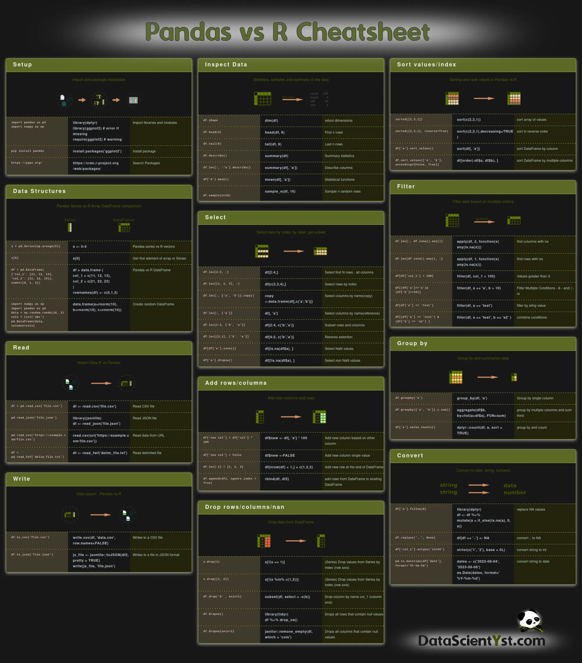
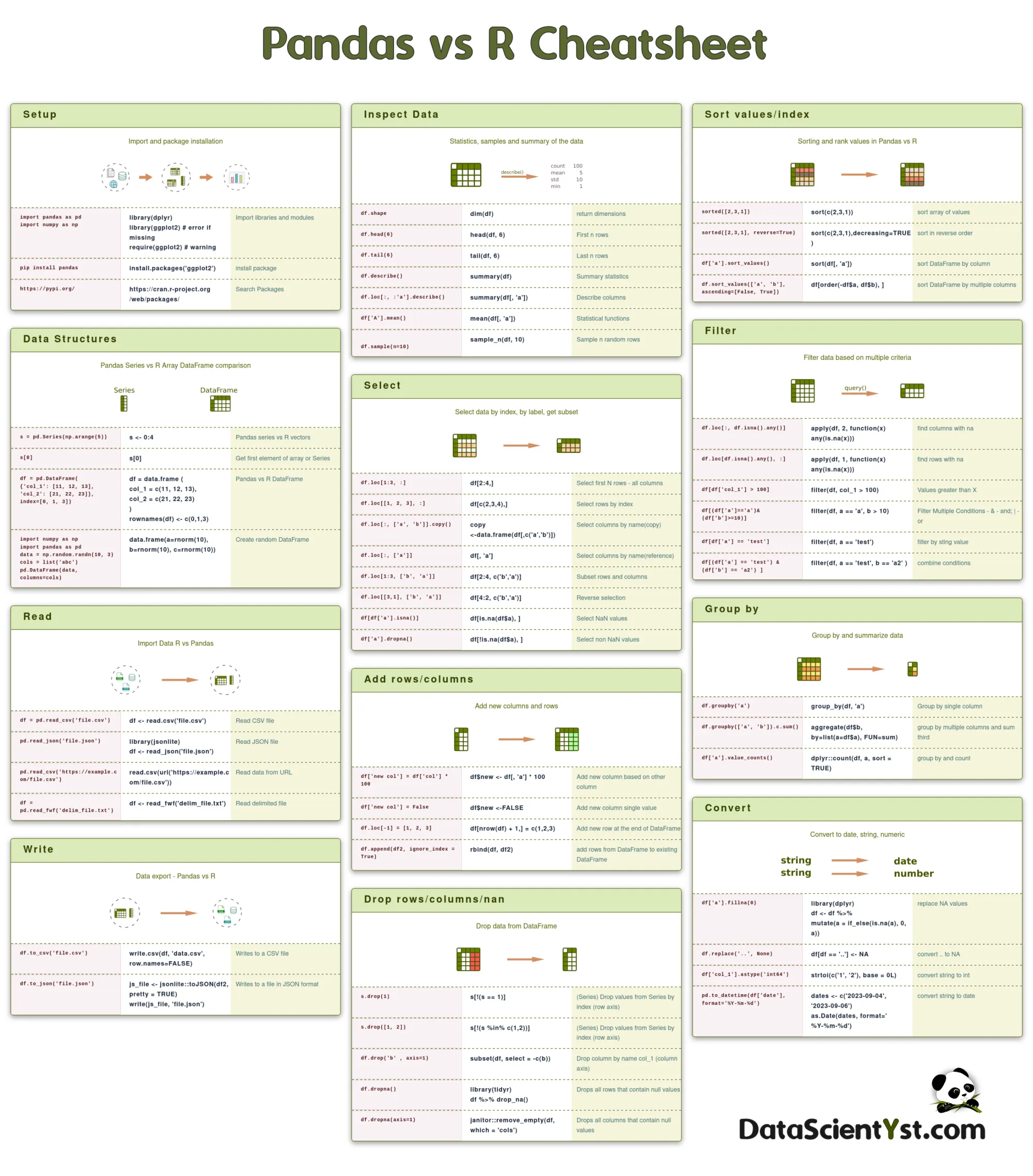
5. Pandas vs R Cheat Sheet Image

Dark version:

Light Version:

6. Pandas vs R comparison

We are working on a visual comparison between R and Pandas. Below you can find a quick teaser:

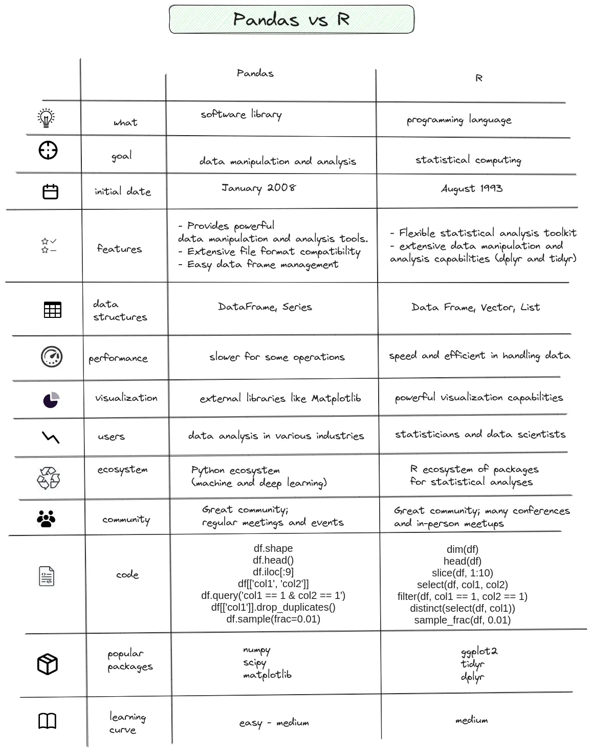
P.S. We were overloaded in the last year so we were not able to post frequently. We hope to have more time for this project and data science.